Boundaries in Physics, and Natural Kinds
Direct Link to File. 1757 words, 9 minute read, 6 paperback pages
C.,
Your previous writing has impressed upon me in a couple ways.
One is just the ‘daunting’ aspect of the knowledge that people in the recent past have still been thinking so specifically about natural kinds as to produce entire edited volumes on the topic!
The other way is, it has made me think about boundary (/ transition) phenomena in natural systems, and their ‘sensitivity’ to ‘noise’. This is related to one of the central themes of my book-idea, that classifications (can) produce discontinuous outcomes. On that topic, I’d previously been thinking about ‘human’ systems, such as sentencing in criminal justice, or giving awards to people who receive certain scores on tests (the original area of investigation for the topic of ‘regression discontinuity design’.
But given that I’m a physicist ;-), it would probably be useful (from an ‘authority’ standpoint) to also talk about natural systems.
Examples that come to mind are the chaos arising in magnetic pendulums; thermodynamic phase transitions; and the ‘comparator’ electronic circuit that we teach in PHY2250, which has a sensitivity to noise necessitating the Schmitt Trigger.
The relevance for machine learning is the following: I have intended to argue that the (location of the) boundary obtained for a classification task is dependent on both the training dataset and the method used. Thus different ‘inputs’ (…I need a better word that ‘input’ that would also encompass the method used; I’m open to suggestions) will give rise to different boundary locations. This is in some sense similar to the in magnetic pendula, in that chaos is usually described in terms of a sensitivity to initial conditions. (You can have chaos without discontinuities, or with discontinuities). And statisticians often speak of ‘noise’ in their datasets, which reminds me of the comparator & Schmitt Trigger.
(It might sound compelling to somehow claim that classification boundaries can introduce ‘chaos’ into systems of human classification, but I would be wary of trying to do that; I think this would be reckless until I think about it more.)
Thus this line of thinking has produced at least these three outcomes for me:
-
Natural kinds exist. ….uh…hahah, ok, that may be question-begging. “Natural phenomena exhibit discontinuous types of behavior that we humans then observe, recognize, and label as being of different kinds” sounds a bit pedantic though.
— What do you think about that?
…the ‘objectivity’ in physics is perhaps easier to make a case for than in biology. (this is true for many assertions about science, not just natural kinds.)
-
The discussion of such natural phenomena in physics makes me feel slightly better about always seeming to be a complete outsider to so much of what we study.
-
The book “Chaos” by James Gleick was an international bestseller and may serve as an inspiration for writing high-popular-level nonfiction. In a like manner, I can perhaps structure the book as being a “tour of” various classification-related phenomena, rather than having the book being structured around some “main point”.
That’s all I’ve got for now. I’m going to save this email in my private blog and resume writing about either patterns or rules.
Best wishes,
Dr. Hawley
PS- I like ‘science toys’ so I looked up ‘magnetic pendulum’ on eBay and immediately found a bunch of ‘magnetic decision maker’ desktop toys! (image below) This is akin to a “Magic 8 Ball” or even just rolling dice – a conversion of continuous-to-discrete behavior that has been used for millennia to influence decision-making! 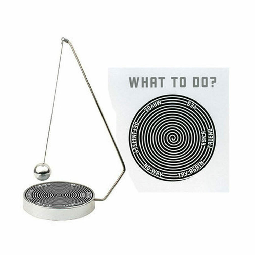
Another example would just be a wheel that you spin, like “Wheel of Fortune” or throwing darts at a target with discrete regions marked with different choices.
“…different ‘conclusions’ that you could ‘jump to’” – Office Space

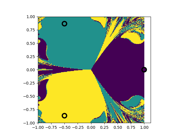
Regions of Decision for Pendulum
So tonight I went ahead an wrote a program to show what the ‘decision boundary’ for a magnetic pendulum starting at rest looks like. I actually did a charged-electrostatic pendulum because I didn’t feel like doing the magnetic field stuff. The results were highly dependent on the parameters of the run, such as the time step, the amount of dissipation, etc. – as one would expect for a chaotic system. Here’s one example of what I got, for a resolution of 250x250:
Code pasted below. And more…
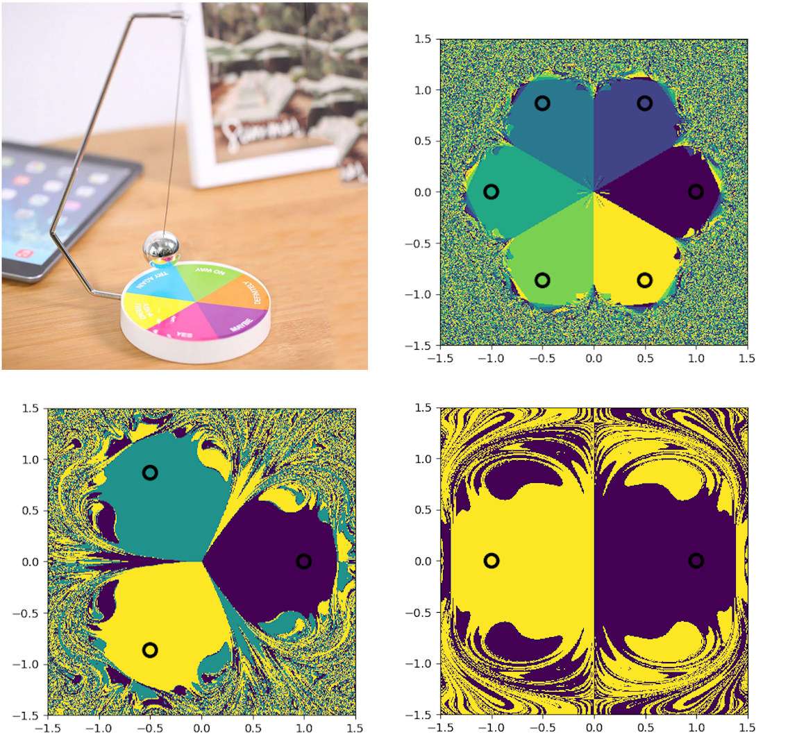
Scrapbooking: Plotting Decision Regions
Starting writing a simulator for a chaotic pendulum. And this came up while I was searching for plotting functions.:
https://rasbt.github.io/mlxtend/user_guide/plotting/plot_decision_regions/
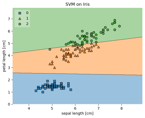
And a related post from Jason Brownlee: https://machinelearningmastery.com/plot-a-decision-surface-for-machine-learning/. TL/DR: Train model on labeled data, make a grid of new input data points, predict on all of them using trained model, then do a contour plot of grid of predictions.
Pendulum sim code
#! /usr/bin/env python
'''
Simulation of a 'magnetic' pendulum. Actually we'll just use
electrostatic charges instead of magnets, but..good enough, right?

Plots an image showing which source the object is closest to after a certain time
(Note: Depending on params like maxiter, the object may still be moving at the
end of the simulation, so the 'ending position' may not be where it comes to rest.)

This code integrates all the (non-interacting) test objects at once, on the GPU.
Uses Beeman algorithm for time integration.

Author: Scott H. Hawley, @drscotthawley
Date: Aug 11, 2020
License: Creative Commons
'''
import numpy as np
import cupy as cp    # cupy is numpy for the GPU
import matplotlib.pyplot as plt


# setup parameters
n_sources = 3      # number of 'magnets', placed evenly around unit circle
res = 256          # image resolution along edges, use multiple of 8 for speed
source_q = -1      # sign of charges. e.g., 1 = repulsive, -1 = attractive


batch_size = res**2   # number of array-based caculations to do at a time


def get_closest(pos, source_pos):
    """
    Find out the source to which each object is closest.
    After many array-shape broadcasting difficulties, I gave up and used a
    loop over sources and a temp storage array. If there's a way to
    do this without that, let me know.
    But, this routine only gets called once, at the end of the simulation,
    so no big deal.
    """
    dist_array = cp.zeros((batch_size, n_sources))  # store dist^2 to each source
    for s in range(n_sources):
        dist_array[:,s] = ((pos - source_pos[s])**2).sum(axis=1)
    return cp.argmin(dist_array,axis=1)             # argmin picks closest


def calc_accel(pos, vel, source_pos, source_charge, accel,
    friction=0.2, eps=0.1, q=1.0, m=1.0, ell=1.0, g=1.0):
    """
    Called by sim_charges.  Calculates acceleration
    Note accel is a tmp array, pre-allocated

        eps:            smoothing parameter to avoid singularity at sources; 'radius of source'
        friction:       coefficient of friction, assuming force is linear w/ velocity
        q:              charge on test charge, in units where physical constants = 1
        m:              mass of test charge
        ell:            length of pendulum
        g:              force of gravity
    """
    # Calculate force (using 'accel' array)
    accel *= 0                           # zero out the accel tmp array
    # Tried to write this without a loop, all vectorized, but had broadcasting problems
    for s in range(source_pos.shape[0]): # for each source
        dr = pos - source_pos[s]         # vector from object to source
        rsq = (dr**2).sum(axis=-1)       # distance squared
        dr_hat = (dr.T / cp.sqrt(rsq))   # .T's are just for broadcasting
        accel += source_charge[s] * q * (dr_hat / (rsq+eps)).T

    accel += -m*g*ell*pos    # Centering force: small angle approx = "spring"
    accel += -friction*vel   # Friction force

    return accel/m   # convert force to accel and return


def sim_charges(pos_0, source_pos, source_charge, maxiter=50000, dt=5e-4):
    """
    Simulate motion of test mass(s) from initial conditions until some stopping
    criterion is met, e.g. max number of iterations.
    This function is designed to simulate an entire 'image' worth of
    (non-interacting) charges.

    Inputs:
        pos_list:       list of all starting positions
        source_pos:     positions (x,y) of each source
        source_charge:  charges of sources
        maxiter:        number of iterations to perform, 'a really long time'
        dt:             time step size

    Outputs:
        2D array of values showing which source each object is closest to
        at end of simulation. Note: no guarantee objects are at rest, so maxiter
        should be large.

    Let's use the time integration algorithm of Beeman, with a predictor-corrector
       for velocity.
       https://en.wikipedia.org/wiki/Beeman%27s_algorithm#Predictor%E2%80%93corrector_modifications
    """
    pos, vel = pos_0, pos_0*0            # start position, from rest

    accel = cp.zeros((batch_size,2))     # allocate storage for acceleration (in x & y)
    new_accel = cp.zeros((batch_size,2))
    accel = calc_accel(pos, vel, source_pos, source_charge, accel) # force at init

    # Startup, first iteration in time
    new_vel  = vel + dt * accel
    new_pos  = pos + dt * (new_vel + vel)/2   # use mean velocty for slightly better acc.
    new_accel = calc_accel(new_pos, new_vel, source_pos, source_charge, new_accel)

    # cycle times and iterations
    prev_pos, prev_vel, prev_accel = pos, vel, accel
    pos, vel, accel                = new_pos, new_vel, new_accel

    # Later time integration
    status_every = maxiter//100          # for printing % progress
    for i in range(maxiter-1):

        # Status message (% Progress)
        if 0 == i % status_every:
            print(f"\r{int(i/maxiter*100):2d}% ",end="",flush=True)

        # Beeman update (predictor-corrector for velocity)
        new_pos = pos + vel*dt + (1./6)*(4*accel - prev_accel)*dt**2
        new_vel = vel + 0.5*(3*accel - prev_accel)*dt    # predictor
        new_accel = calc_accel(new_pos, new_vel, source_pos, source_charge, new_accel)
        new_vel = vel + (1./12)*(5*new_accel + 8*accel - prev_accel)*dt # corrector

        # cycle times and iterations
        prev_pos, prev_vel, prev_accl = pos, vel, accel
        pos, vel, accel               = new_pos, new_vel, new_accel

    print("")

    # after loop, use final position for 'color'
    img_vals = get_closest(pos, source_pos)
    #img_vals = cp.sqrt((vel**2).sum(axis=-1)) # color using final speed instead

    img_vals = cp.reshape(img_vals,(res,res))  # convert from long list to 2D

    return img_vals.T       # .T b/c numpy/cupy axes are 'backwards' wrt images


#### Main code starts here #####

print(f"Image resolution will be {res}x{res}")

# Place sources equally around unit circle, starting along x axis
thetas = cp.linspace(0, 2*cp.pi, num=n_sources+1)[0:-1]
#print("Thetas (deg) = ",thetas*180/cp.pi)
source_pos = cp.vstack((cp.cos(thetas),cp.sin(thetas))).T
source_charge = source_q * cp.ones(n_sources)  # equal charges for sources
print("Sources located at\n",source_pos)

# Generate a long list of starting positions
x = y = np.linspace(-1.5, 1.5, res)            # Use numpy not cupy here!
pos_start = cp.array([[x[i],y[j]] for i in range(res) for j in range(res)])

# Fill the image
print(f"Simulating motion of all test objects...")
z = sim_charges(pos_start, source_pos, source_charge)

# Bring arrays back to CPU for plotting
z, source_pos = cp.asnumpy(z), cp.asnumpy(source_pos)

# Plot results
print("Plotting the image")
fig, ax = plt.subplots()
cmap = plt.cm.viridis   # good for colorblind peeps & converts to greyscale well
cs = ax.pcolor(x, y, z, cmap=cmap)
plt.gca().set_aspect('equal', adjustable='box')
#fig.colorbar(cs, ax=ax)      # if you want a color bar

# Show the locations of the sources, with black circles around them
ax.scatter(source_pos[:,0],source_pos[:,1], s=60*2, linewidths=3,
    edgecolors='black', c=range(n_sources), cmap=cmap)

filename = f'pendulum_image_{res}_{n_sources}_{np.int(source_q)}.png'
print(f"Saving image to {filename}")
plt.savefig(filename, dpi=200)
plt.close(plt.gcf())

print("Finished.")